Check Lightcurve for Solar System Contamination

When collecting time series observations of stars near the ecliptic plane, often solar system objects can wander in and out of the field of view. This in principle could affect a transit or flare searches, either by contaminating the aperture (making the star appear temporilly brighter) or the background (making the star appear temporarily dimmer). We can use jorbit and its pre-computed ephemerides to check for the impact of solar system objects on a lightcurve.

import numpy as np
import matplotlib.pyplot as plt
import astropy.units as u
from astropy.coordinates import SkyCoord
from astropy.time import Time

from jorbit.mpchecker import nearest_asteroid, animate_region

If we want just a quick/easy check if any solar system objects are in the field of view, we can run:

separations, asteroids = nearest_asteroid(
    coordinate=SkyCoord(ra=0 * u.deg, dec=0 * u.deg),
    times=Time("2025-01-01") + np.arange(0, 3, 1 / 24 / 4) * u.day,
    radius=2 * u.arcmin,  # roughly ~10x10 TESS pixels, comparable to a TPF
)

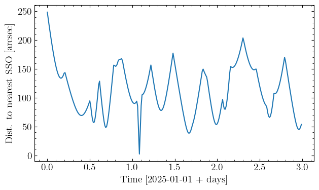
This uses the same assumptions baked into the extra_precision=False version of the mpchecker function, namely a geocentric observer and Newtonian-only gravity. But, it gives us a good first look at what might be happening near our target. separations is now a vector of anglular separations to the nearest solar system object, and asteroids is a Table of all the asteroid that flew within our radius during the times we checked:

fig, ax = plt.subplots()
ax.plot(np.arange(0, 3, 1 / 24 / 4), separations)
ax.set(xlabel="Time [2025-01-01 + days]", ylabel="Dist. to nearest SSO [arcsec]");

asteroids

Table length=15

Unpacked Name	Packed designation	H	G	Epoch	M	Peri	Node	Incl.	e	n	a	U	Reference	#Obs	#Opp	Arc	rms	Coarse Perts	Precise Perts	Computer	Flags	last obs
str19	str7	float64	float64	str5	float64	float64	float64	float64	float64	float64	float64	str1	str9	float64	float64	str9	float64	str3	str3	str8	str4	str8
(126467) 2002 CZ39	C6467	15.68	0.15	K2555	226.25838	346.4117	200.08916	13.12886	0.1046767	0.24252144	2.5466501	0	E2025-B02	758.0	18.0	2000-2025	0.8	M-v	3Ek	MPCLINUX	0000	20250116
(180961) 2005 MJ35	I0961	17.34	0.15	K2555	132.90427	181.27084	79.88972	0.03589	0.1919256	0.26343893	2.4099947	0	MPO889347	451.0	18.0	1998-2024	0.86	M-v	3Ek	MPCLINUX	0000	20241204
(184308) 2005 EY209	I4308	16.51	0.15	K2555	142.98958	61.02093	201.32048	1.47144	0.0313494	0.22644374	2.6658098	0	E2025-B02	497.0	18.0	1998-2025	0.86	M-v	3Ek	MPCLINUX	0000	20250116
2005 UX268	K05UQ8X	20.24	0.15	K2555	77.16673	319.34595	32.85986	22.75135	0.1125138	0.35985207	1.9575824	9	MPO630349	12.0	1.0	1 days	0.51	M-v	3Ek	Pan	2006	20051029
2013 CZ241	K13CO1Z	17.89	0.15	K2555	161.74732	220.42167	19.20711	5.3706	0.0539605	0.21441105	2.7646359	0	E2024-T78	45.0	6.0	2013-2024	0.4	M-v	3Ek	MPCLINUX	0000	20241004
2013 UN46	K13U46N	17.62	0.15	K2555	15.88923	187.81528	202.26333	3.30755	0.188936	0.17419598	3.1752454	0	MPO893404	69.0	6.0	2013-2024	0.43	M-v	3Ek	MPCLINUX	0000	20241204
2015 RP328	K15RW8P	18.35	0.15	K2555	57.63518	323.39622	22.09817	4.49386	0.0783381	0.21568601	2.7537303	0	E2024-SF9	31.0	4.0	2015-2024	0.71	M-v	3Ek	MPCLINUX	0000	20240928
2016 BK84	K16B84K	17.32	0.15	K2555	255.37314	140.798	15.97159	10.97567	0.172949	0.17929154	3.1147953	0	E2024-TN4	84.0	7.0	2010-2024	0.42	M-v	3Ek	MPCLINUX	0000	20241010
2016 DA31	K16D31A	29.9	0.15	K2555	199.17288	272.94207	336.96023	0.02153	0.4435599	0.715656	1.2378457	8	MPO377910	14.0	1.0	1 days	0.44	M-v	3Eh	MPCW	2803	20160229
2016 UR162	K16UG2R	18.8	0.15	K2555	102.20193	264.35742	22.83458	2.95894	0.1859327	0.23757626	2.5818679	8	MPO660523	24.0	1.0	3 days	0.21	M-v	38h	Veres	2000	20161029
2023 XQ16	K23X16Q	30.58	0.15	K2555	158.79242	133.51724	257.97903	1.22932	0.069156	0.93444997	1.0361724	5	E2024-C37	40.0	1.0	3 days	0.48	M-v	3Ek	MPCLINUX	2803	20231218
(346625) 2008 WK112	Y6625	17.43	0.15	K2555	37.24264	346.58397	28.74814	1.58445	0.2097466	0.23972584	2.5664107	0	E2024-V47	403.0	15.0	2001-2024	0.9	M-v	3Ek	MPCLINUX	0000	20241102
(371405) 2006 RN84	b1405	18.11	0.15	K2555	22.04551	195.89265	210.51482	0.78697	0.179655	0.27195746	2.3594026	0	E2024-U19	218.0	11.0	2006-2024	0.96	M-v	3Ek	MPCLINUX	0000	20241018
(492869) 2014 QN378	n2869	17.38	0.15	K2555	77.61079	119.11664	200.28638	5.29788	0.0737311	0.19636474	2.9315257	0	MPO891620	116.0	12.0	2004-2024	1.04	M-v	3Ek	MPCLINUX	0000	20241204
(610939) 2006 KB148	z0939	17.69	0.15	K2555	278.59983	301.22169	200.96289	12.21888	0.10554	0.24048836	2.5609829	0	E2024-UB5	93.0	8.0	2006-2024	0.45	M-v	3Ek	MPCLINUX	0000	20241024

Looks like there was a close approach by something moving rapidly around one day into our time series. To investigate its potential impact on our lightcurve, we can run:

separations, asteroids, coord_table, mag_table, total_mags = nearest_asteroid(
    coordinate=SkyCoord(ra=0 * u.deg, dec=0 * u.deg),
    times=Time("2025-01-01") + np.arange(0, 3, 1 / 24 / 4) * u.day,
    radius=2 * u.arcmin,
    compute_contamination=True,
    observer="geocentric",
)

Note that now we’ve set compute_contamination=True and specified a specific observer, which initiates several extra calculations, again like the extra_precision=True version of mpchecker. This takes considerably longer (this ~300 point time series takes ~a min on my laptop), but a lot is happening behind the scenes: we’re running the initial low precision version to flag all the relevant asteroids, running an N-body simulation to map each one to each moment in our time series, then computing its sky position and estimated magntidue as seen from a particular observer.

We can now look at a time series of the total magnitude of all asteroids in our field of view:

fig, ax = plt.subplots()
ax.plot(np.arange(0, 3, 1 / 24 / 4), total_mags)
ax.set(xlabel="Time [2025-01-01 + days]", ylabel="Total V Mag from SSOs");

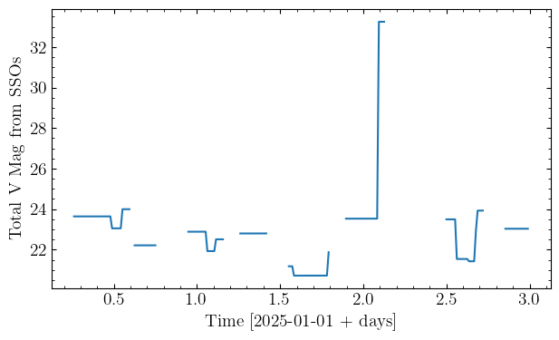
This shows us that although the separation might have been small, the magnitude of the object was very faint, and so it likely had little impact on our lightcurve. The gaps here correspond to times when nothing fell within our search radius, meaning the magnitude was technially $\infty$. Finally, for fun and a sanity check, we can animate what was happening in the sky using the outputs of the above function:

anim = animate_region(
    coordinate=SkyCoord(ra=0 * u.deg, dec=0 * u.deg),
    times=Time("2025-01-01") + np.arange(0, 3, 1 / 24 / 4) * u.day,
    coord_table=coord_table,
    radius=2 * u.arcmin,
)

Once Loop Reflect

This should render within a notebook, but can also be saved as a gif via something like:

anim.save('animation.gif', writer='pillow')